Statistics

In this lecture we will see how to apply statistics and probability to find the probability that a hypothesis is true based on data. The mathematics we will cover is the fundamentals of statistics for experimental research.

This lecture aims to give you an intuitive understanding of why inferential statistical tests work the way they do and to give you practical tools for you to use for planning and analysing your own research.

Mathematics and Problem Solving

12. Inferential Statistics

David Gundry

Introduction

Inferential statistics allow us to make inferences from a sample of data. Most often this takes the form of a hypothesis test: we collect some data to infer whether a given hypothesis is likely to be true.

The fundamental problem of statistics is that we want to describe a population of potential measurements based on a limited amount of data. As it is impractical or impossible to collect all the data we might need, we need to make judgements based on probability.

For most types of quantitative research we start by collecting data from a sample that is representative of the population. We perform some statistical analysis on that data in order to generalise our findings from the sample to the wider population with some level of confidence. As we cannot be sure that the results of our sample are the same as for the overall population that it is meant to represent, we express our results in terms of probabilities. We use inferential statistics to allow us to make these generalisations based on sound mathematical principles.

Any inferential statistical analysis relies on certain assumptions being correct. One necessary assumption is that the sample is representative of the population. We usually need to assume that the population was sampled at random, meaning each individual has an equal chance of being included in the sample. When we interpret the results of a statistical test, we need to make sure we understand the assumptions that it makes and be able to judge whether these assumptions are reasonable.

Generalisation from a Sample

Learning Outcomes

Calculate and interpret basic inferential test statistics

Calculate the z statistic
Calculate the t statistic
Interpret test statistic in comparison to critical values

Select an appropriate statistical test

Learning Outcomes

Calculate and interpret basic inferential test statistics
Select an appropriate statistical test

Overview

We will start by familiarising ourselves with the core concepts and terminology that are used in inferential statistics. We will then build an intuitive understanding of how inferential statistical tests by unpacking two basic statistical tests, the Z test and the Student's T test. Finally we will discuss how to choose between different inferential statistics.

Overview

Core Concepts
Understanding Inferential Statistics
Choosing Inferential Statistics

Core Concepts

Sample

The data that we use for inferential statistics comes from a sample of a wider population. For this sample, we can calculate various statistics.Where our sampled variable is drawn from a normal distribution, we require the mean and the standard deviation of the sample, as this is enough to approximate the probability distribution that the sample came from.

Sample

We sample data $x$ from the population

We calculate descriptive statistics such as

group mean $\overset{―}{x}$
sample standard deviation $s_{x}$

Hypothesis

Our goal is to support or refute particular claims about the world (or the system under test). These claims take the form of hypotheses. Hypotheses can be understood in terms of probability as disjoint (mutually exclusive) events.

We have one (or more) alternate hypotheses that describes the situation or event we are expecting to find/observe. In addition to our alternate hypotheses, we state a null hypothesis which describes the situation or event in which there is no effect, no difference, or nothing unusual is going on.

For example, imagine that we are investigating the intelligence of bears and we have a particular bear who we think is pretty clever. To turn this into a testable hypothesis, we would state the hypothesis that our bear is smarter than the average bear. This is our alternate hypothesis - the effect we are expecting to find. Our null hypothesis would be that there is no difference in intelligence between our bear and the average bear.

Most hypotheses are of the form that such-and-such a group or such-and-such an individual differ on some variable compared to the wider population, or that two groups are different from each other on some variable. In terms of probability distributions, we are asking whether the samples are likely to be drawn from the same probability distribution, or whether they likely come from different probability distributions.

Hypothesis

We want to evaluate which of two disjoint events (hypotheses) is true:

$H_{0}$ - Null Hypothesis

$H_{1}$ - Alternate Hypotheses

Do samples come from the same ( $H_{0}$ ) or different ( $H_{1}$ ) probability distributions?

Test Statistic

Most inferential statistics test for differences between two or more sets of data. However, what counts as a difference? It is not enough to test whether there is a difference, because small differences are likely to arise due to chance variation. Rather than saying how big the difference is, we want to say how unexpected it is. Inferential test statistics express how unexpected an observed difference is.

Each test statistic is expressed on a different scale, and they cannot be directly compared. To interpret an inferential statistic, we consider the probability distribution of that test statistic. We calculate the probability of observing a test statistic of at least that size.

Test Statistic

Inferential test statistics reflect how interesting a difference is, e.g.

$z$ (Z test)
$t$ (T test)
$F$ (ANOVA)

Test statistics are interpreted based on their probability distribution

P Value

The result at the end of our statistical analysis is a $p$ value. We get a $p$ value for each hypothesis test / inferential statistic we calculate. This is the primary value that we use to decide whether to reject our null hypothesis. It is also one of the most important statistics to report.

The $p$ value describes the probability that the results we observed were the result of chance. As it is a probability, so it must always be in the range $0 < p < 1$ .

The $p$ value gives us the likelihood of making a Type 1 Error. This type of error is a false positive - where we conclude there is an effect when there is no effect.

The $p$ value is calculated from test statistic and degrees of freedom.

P value

We use $p$ for the probability an effect observed is due to chance variation

Type I Error

Falsely rejecting the null hypothesis

If $p = 0.05$ , we have a 5% chance of making a Type I error.

Alpha

The $p$ value is compared against a significance level to decide whether the chance that we have observed an effect is large enough to conclude that we really have observed an effect. We must set the significance level for each statistical test we conduct. Typically this value is no larger than $p = 0.05$ , meaning it is normal to conclude that we have observed an effect when there is less than a 5% chance of a false positive.

If the $.05$ level is achieved ( $p$ is equal to or less than $.05$ ), then a researcher rejects the $H_{0}$ and accepts $H_{1}$ . If the $.05$ significance level is not achieved, then the $H_{0}$ is retained

Alpha

We use $α$ to label our significance threshold. Alpha ( $α$ ) is usually set to 0.05

$p < α$

statistically significant

$p > α$

not statistically significant

Multiple Testing

We can think of calculating a hypothesis test against an alpha (significance level) of 0.05 as like rolling a 20 sided dice. There is a 1 in 20 chance (0.05) of rolling a 20. Here rolling a 20 represents the situation where we have a false positive - where we incorrectly conclude that we observed an effect.

From probability, we can calculate that the probability of getting at least one 20 if we roll the dice twice as being $0.05 + 0.05 - (0.05 \times 0.05) = 0.0975$ . This is almost double the chance of getting a 20 if we roll the dice only once! The probability of getting at least one 20 increases for every time we roll the dice. Similarly, with hypothesis testing, the probability of getting at least one false positive increases with every hypothesis test run.

In any situation where we are testing (effectively) the same hypothesis multiple times - and where we would report having detected an effect based on any individual test finding an effect - we need to reduce our alpha to adjust for this increased probability of a type 1 error (false positive). (This is also why it is important for null results to be published - if only positive results are published, there will be an inflated false-positive rate.)

Multiple Testing

Consider two hypothesis tests

Each test $n$ has probability of type-1 error $P (E_{n}) = α$

P (E_{1} \cup E_{2}) = P (E_{1}) + P (E_{2}) - P (E_{1} \cap E_{2})

Experiment-wise type 1 error rate is inflated in multiple testing

Bonferoni Correction

For $m$ hypothesis tests, adjusted alpha is set to $\frac{α}{m}$

Degrees of Freedom

The degrees of freedom for a statistic is the number of values used in its calculation that would be able to vary without changing the value of the statistic itself. This can be confusing to understand, so let's consider a simple example with the calculation of the arithmetic mean of a sample of four numbers:

(3 + 4 + 6 + 7) / 4 = 5

Here we have four values, or data points, involved in the calculation: 3,4,6, and 7. Were we to report the mean of this set of numbers (which as we can see is 5), we could say that the mean is 5, and there are 3 degrees of freedom. To understand why there are three degrees of freedom, you need to imagine for a moment that you do not know what data this statistic was calculated from.

Now assuming that you know that the mean is 5, and that the sample size was 4 (i.e., we found the mean of four numbers) only three of the four data points are free to vary independently. This is because while three of the values could have been any number, the fourth value is completely determined by the previous three and the mean. In other words, If I gave you three values and the mean, you could work out the fourth value. Algebraically, you can see this as the following problem, where you can solve for $x$ :

(3 + 4 + 6 + x) / 4 = 5

Thus the value of $x$ in this case is not free to vary, but is completely specified by the other values. There are three remaining data points that are free to vary, thus our mean has three degrees of freedom, written 3 d.f.

$d.f.$ affects the interpretation of some statistics. There are rules for how to calculate d.f. for each statistical test

Degrees of Freedom

Degrees of freedom ( $d.f.$ ) give the number of values that could vary in the calculation of a statistic

Related to sample size

Example

In calculating mean, there are $n - 1$ degrees of freedom, as one value is completely determined, e.g.:

(3 + 4 + 6 + x) / 4 = 5

Question

Example

In a study, mean scores for an HCI usability scale are calculated for men and women. The null hypothesis is that there is no difference in gender in perceived usability of a certain website.

$p = .12$ , $α = .10$ , $t = 1.8$ $d = 0.32$

Question

Would we accept or reject the null hypothesis?

Understanding Inferential Statistics

Basic Intuition

A basic inferential statistic is the ratio between the difference we observed compared to the typical difference we would expect. The larger the difference we observe is relative to what we would expect, the larger our inferential statistic.

The observed and expected values vary depending on our experiment. We might be testing whether an individual is significantly different from a group. In which case our observed value would be the individual measurement, and the expected value would be the group mean. This makes the observed difference the difference between our individual and the group.

The typical difference is also called the standard error, and we will see some examples of how it is calculated for different probability distributions below.

Basic Intuition

Inferential statistics express the difference between 2 numbers:

\frac{observed - expected}{typical difference}

Observed

Measurement ( $x$ )
Mean ( $\overset{―}{x}$ )
Difference between groups ( $\overset{―}{x} - \overset{―}{y}$ )

Expected

Group mean ( $\overset{―}{x}$ )
Population mean ( $μ$ )
No difference ( $0$ )

Fish Example

Imagine we know that on average fish are 150 units long. We measure a fish and find it is 175 units long. We can calculate the difference that we have observed by comparing what we observed (175) to what we expected (150).

175 - 150 = 25

We have a difference of 25, but to determine whether this difference is interesting we must compare it against the typical differences in fish size. We need to know the variance in measurements of fish size

Let us assume

μ = 150 σ = 10

Then 175 is over 2 standard deviations away from mean. As 95% of data is within 2 standard deviations of mean, that makes our fish in at least the most extreme 5% of fish sizes. Interesting fish!

(Fish images by Vecteezy)

Sampling Distributions

The sampling distribution is the statistical distribution that your observed value comes from. For example if we sample individuals, our sampling distribution is the same as our population distribution. In the example above, we sampled individual fish, so our sampling distribution was the same as our population distribution, which was a normal distribution.

However, often the observed value is not an individual measurement, but the mean of a group of measurements. Means of values drawn from a given distribution have a different distribution to the values themselves. Consider that it is much more likely to get a single extreme value than to average several values and get an extreme value for the mean. Therefore, when we sample group means of size $n$ , our sampling distribution is a distribution of means of groups of size $n$ .

According to the Central Limit Theorem, for large sample sizes, the sampling distribution for means approximates a normal distribution with a mean equal to the population mean, and a standard deviation equal to $\frac{σ}{\sqrt{n}}$ . This applies even when the population distribution is not itself normal.

Sampling Distribution

The sampling distribution is the distribution from which the observation is drawn

Individual Value

Same as population distribution, e.g. normal for given $μ, σ$

Group Mean

Distribution of group means of size $n$ for a given $μ, σ$

Standard Error

Standard error is the standard deviation of our sampling distribution. For our fish example, our standard error would be the standard deviation of our data (assuming our individuals are normally distributed).

When comparing group means, we need to adjust our standard error as our sampling distribution is no longer normal. It is a distribution formed of means of groups of size $n$ . The standard deviation of this distribution is our original $σ$ divided by the square root of the group size. We can still calculate a $z$ statistic (as it's still in standard deviations).

S E = \frac{σ}{\sqrt{n}}

When comparing differences in group means, again we have a different sampling distribution, so we need a different formula for our standard error:

S E = \sqrt{\frac{σ_{1}^{2}}{n_{1}} + \frac{σ_{2}^{2}}{n_{2}}}

Standard Error

Typical difference is the standard deviation of sampling distribution, called standard error

inferential statistic = \frac{observed - expected}{S E}

Individuals

S E = σ

Group Means

S E = \frac{σ}{\sqrt{n}}

Differences in Group Means

S E = \sqrt{\frac{σ_{1}^{2}}{n_{1}} + \frac{σ_{2}^{2}}{n_{2}}}

Z Statistic

Let us begin with our basic formula for an inferential statistic:

\frac{observed - expected}{typical difference}

Consider the situation where we observe a single data point and we are comparing it to the population mean. Our observation is of a data point, $x$ . Our expectation would be that the value is the population mean, $μ$ . The typical variation is given by the population standard deviation, $σ$ .

Z Statistic

Compare against a population with given $μ$ , $σ$

Simple Z test

Single value $x$

z = \frac{x - μ}{σ}

One-sample Z Test

Sample mean $\overset{―}{x}$

z = \frac{\overset{―}{x} - μ}{\frac{σ}{\sqrt{n}}}

Two-sample Z test

Population means $μ_{1}$ and $μ_{2}$

z = \frac{(μ_{1} - μ_{2}) - 0}{\sqrt{\frac{σ_{1}^{2}}{n_{1}} + \frac{σ_{2}^{2}}{n_{2}}}}

Z Distribution

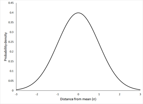
Imagine we randomly sampled a normal distribution and calculated z statistics for single values, for samples, or for comparing two sample means using the $z$ statistic formulas above. We could then plot the probability distribution that the z statistic follows. This is called the $z$ distribution.

If we generate a random $z$ statistic - i.e. we perform a random hypothesis test - we might expect that the majority of the time we are going to see a small value for $z$ , because we sampled from our population distribution. This is because most of the time differences that we observe between our sample mean and the population mean are going to be small. Extreme values for $z$ are going to be uncommon, because we only get a large value for z when we happened to have selected a sample with an unusually large or small mean.

As it happens, the $z$ distribution is a normal distribution. The mean is 0 (because the average difference that we would observe between sample and mean is 0). The standard deviation is 1.

Now we can compare the value we have computed for $z$ , and calculate the probability that we would observe that value by chance. If the probability is low, that suggests it is unlikely that our observation (which we used to calculate $z$ ) is drawn from the population distribution, the value is likely drawn from some other distribution. In other words, where the probability of getting our $z$ value is low, it is likely because our sample is significantly different to the population.

Z Distribution

Probability density of getting a particular $z$ value by chance

Normal distribution with $μ = 1$ , $σ = 1$

T Statistic

We rarely know the population standard deviation, and thus we cannot often use a $z$ test. More often, we know the standard deviation of a sample. This standard deviation is only an approximation - though the larger the sample size used to calculate the standard deviation, the better that approximation is.

Because of the error inherent in using an approximation of standard deviation, the values that we derive are different. This is most evident when sample sizes are smaller than 30. When we use the approximation of standard deviation, the resulting statistic is called a $t$ statistic.

Like Z tests, T tests assume data follows a normal distribution. This makes it a parametric test. It similarly assumes representative, randomly selected samples and similar variance between groups.

T Statistic

Assume normal distribution, but $σ$ is unknown

One-sample t test

Compare sample with given $\overset{―}{x}$ , $s$

t = \frac{\overset{―}{y} - μ}{\frac{s}{\sqrt{n}}}

Two-sample t test

Compare the mean of two samples $x_{1}$ and $x_{2}$

t = \frac{(\overset{―}{x_{1}} - \overset{―}{x_{2}}) - 0}{\sqrt{\frac{s_{1}^{2}}{n_{1}} + \frac{s_{2}^{2}}{n_{2}}}}

T Distribution

As the $t$ statistic is calculated with an approximation of standard deviation that depends on sample size (which is closely related to degrees of freedom), the $t$ distribution is dependent on the number of degrees of freedom in the calculation.

When the distribution of the $t$ statistic for a given sample size is plotted, we see that, where degrees of freedom are low, the distribution has thicker tails. When the degrees of freedom are high, the distribution approximates the $z$ distribution.

(Note: In the interactive example embedded on the slides, $v$ is degrees of freedom)

T Distribution

The $t$ statistic uses $s$ , which only approximates $σ$

Sample Standard Deviation

s = \sqrt{\frac{\sum_{i = 1}^{n} (x_{i} - \overset{―}{x})^{2}}{n - 1}}

Population Standard Deviation

σ = \sqrt{\frac{\sum_{i = 1}^{n} (x_{i} - \overset{―}{x})^{2}}{n}}

The $t$ distribution approximates a normal distribution for large $n$

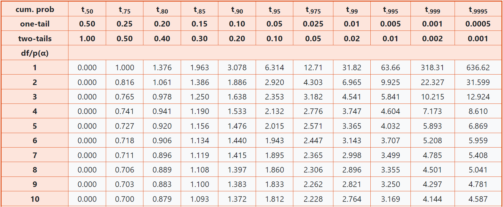
Critical Thresholds

For each test statistic, we can calculate the value that corresponds to a particular probability. For example, we can calculate the z statistic where the probability of generating a value at least as extreme as it is 0.05. If our significance level is set to 0.05, we are able to compare our calculated $z$ against this value to check if our result is significant at the 0.05 level.

Find t tables at t-tables.net

Critical Thresholds

Compare your inferential statistic (e.g. $z$ , $t$ ) against a critical threshold to test for statistical significance, e.g.

Effect Size

Effect size is usually calculated using the formula for Cohen's $d$ .

d = \frac{\overset{―}{x} - \overset{―}{y}}{s_{p o o l e d}}

This is the observed difference between the samples as a proportion of the standard deviation. If the standard deviation varies between groups, the pooled standard deviation must be used:

s_{p o o l e d} = \sqrt{\frac{s_{1}^{2} + s_{2}^{2}}{2}}

Where $s_{1}$ and $s_{2}$ are the standard deviations of $x$ and $y$ respectively.

Effect size is a unitless measure that can be used to compare the effect sizes of different studies. A very approximate rule of thumb - where there is no more specific data available is:

Cohen's $d$	Description
0.2	Small
0.5	Medium
0.8	Large

Effect Size

How large is the difference between conditions?

significance $⇏$ importance

Cohen's $d$ expresses observed difference as a proportion of typical difference

d = \frac{\overset{―}{x_{1}} - \overset{―}{x_{2}}}{\sqrt{\frac{s_{1}^{2} + s_{2}^{2}}{2}}}

Inferential Statistics: 5 Steps

To determine if sample means come from same population, use 5 steps with inferential statistic

1. State Hypothesis

$H_{0}$ : there is no difference between 2 means; any difference found is due to sampling error

$H_{1}$ : there is a difference between the two means; the samples are drawn from different distributions.

Results are stated in terms of probability that $H_{0}$ is false. Usually the goal of a study is to reject $H_{0}$ .

2. Level of Significance

Decide on the alpha level, or level of significance. This is the probability of observing a result by chance, or observing a result if two samples were drawn from the same population. This is usually set to $α = 0.05$ . The smaller the value of $α$ the more confidence we require to conclude that we have found a true effect.

3. Computing Test Statistic

Use a statistical test formula to derive an appropriate test statistic (e.g. $z$ value, $t$ value, or $F$ value). We need to select a test statistic based on appropriate assumptions about our data.

4. Obtain Critical Value

A value derived from the test statistic distribution for a given number of degrees of freedom, and the significance level $α$ . We compare our calculated test statistic to this critical value to determine if findings are significant. If our test statistic is larger than the critical value, we reject $H_{0}$ .

5. Reject or Fail to Reject $H_{0}$

Calculated value is compared to the critical value to determine if the difference is significant enough to reject Ho at the predetermined level of significance

If test statistic is greater than the critical value then we reject $H_{0}$ . If test statistic is less than the critical value then we fail to reject $H_{0}$ . Rejecting $H_{0}$ , supports $H_{1}$ , but it does not prove $H_{1}$ .

Choosing Inferential Statistics

Independent or Paired

Is the data in the two (or more) sets paired, or is every data point independent from every other? i.e. can you match records between the sets? If yes - they are paired. For example a before and after test with the same respondents would be paired data.

Independent or Paired

Independent samples

Group A	Group B
3	2
4	5
2	5
$\overset{―}{A} = 3$	$\overset{―}{B} = 4$

Are $\overset{―}{A}$ and $\overset{―}{B}$ different?

Paired samples

Pre test	Post test	Difference
2	3	1
4	6	2
2	5	3
		$\overset{―}{D} = 2$

Is $\overset{―}{D}$ different to $0$ ?

Parametric or Non-Parametric

Most statistics assume your data are normally distributed. If they are use a parametric test if not use a non-parametric test.

How to decide? Test for normality - use the Shapiro-Wilk or the Kolmogorov-Smirnov test. S-W generally considered to be better.

For both if $p > 0.05$ we assume a normal distribution

Parametric or Non-Parametric

Parametric

Non-Parametric

Any other probability distribution

For nominal or ordinal data

One or Two Tailed

You must decide whether to run a one or a two-tailed test. Ideally this should be a principled decision based on the nature of the hypothesis.

When determining the critical value for a statistic - that is, what value counts as sufficiently unexpected to be deemed statistically significant - you need to decide whether you are looking for values that are either unexpectedly large or small, or whether you are only looking for values that are unexpectedly large, or whether you are only looking for values that are unexpectedly small. In other words, does any extreme value count, or does it only count if it is extreme in a particular direction?

As the significance level is the same (e.g. 0.05) whether you are running a one- or two-tailed test, the critical values will be lower in a one-tailed test than a two-tailed test. As you only will accept positive results in one direction, there is no possibility of you getting a false positive in the other direction. All of the chance of false positives is concentrated on one end.

In the slides you can see two graphs. The first represents a two-tailed test. If the highlighted area adds up to 0.95, there is a 0.05 chance of a number being in one of the tails that are not highlighted. The second graph represents a one-tailed test. Now the area were significance is achieved is concentrated on one side. The critical threshold is thus lower to achieve the same significance level.

Choosing one- or two-tailed tests

Your default choice should be to use a two-tailed test. Even when you have a directed hypothesis, a two-tailed test will be less likely to make a type 1 error (false positive), so it is the conservative option.

However, if you hypothesis that your dependent and independent variables have a clear directional relationship, you might choose to use a one-tailed test. This might be because there are strong theoretical reasons to expect a particular directed result. Or it might be that a result in the direction other than the one you expect would not be meaningful or interesting. For example, if you test whether a game is more enjoyable than a control condition, it might be that finding the opposite (control is more enjoyable than the game) just demonstrates that your study is flawed rather than providing any meaningful conclusions.

You do not need a strong principled reason to use a one-tailed test. However, because significance is easier with a one-tailed test, readers may be suspicious if its use is not justified, particularly if your results only just achieve significance. If you have not pre-registered your analysis, a reader might suspect you chose a one-tailed test only after you saw the direction of the results. Doing this significantly increases the risk of a type 1 error, and is bad statistical practice.

Chi-Squared Test

Used to test whether categorical variables are independent.

Do observed frequencies differ from expected frequencies in a statistically significant way?

A Chi-squared goodness of fit test is used to test whether a set of frequencies differ from a given set of expected frequencies.

A Chi-squared test of independence is used to test whether two independent categorical variables differ significantly from each other.

Chi-Squared test

	A	B	C	Total
Category 1				3
Category 2				3
Total	2	2	2	6

Expected

	A	B	C
Category 1	1.0	1.0	1.0
Category 2	1.0	1.0	1.0

colTotal \times \frac{rowTotal}{overall total}

For each cell, calculate sum of $\frac{(observed - expected)^{2}}{expected}$ . Above $χ^{2} = 0.00$

Which test to use?

Summary

Core concepts

Sample
Hypotheses
Test Statistics
P Value
Alpha (Significance level)

Inferential statistics

Test statistics say how unexpected an observed difference is

test statistic = \frac{observed - expected}{typical difference}

Either

calculate probability from probability distribution of statistic
compare test statistic against critical value

Choosing Inferential Statistics

Independent or paired?
Parametric or non-parametric?
One- or two-tailed?

Statistics

Mathematics and Problem Solving

12. Inferential Statistics

Introduction

Learning Outcomes

Learning Outcomes

Overview

Overview

Core Concepts

Core Concepts

Sample

Sample

Hypothesis

Hypothesis

Test Statistic

Test Statistic

P Value

P value

Type I Error

Alpha

Alpha

p<α

p>α

Multiple Testing

Multiple Testing

Bonferoni Correction

Degrees of Freedom

Degrees of Freedom

Example

Question

Example

Question

Understanding Inferential Statistics

Understanding Inferential Statistics

Basic Intuition

Basic Intuition

Observed

Expected

Fish Example

Sampling Distributions

Sampling Distribution

Individual Value

Group Mean

Standard Error

Standard Error

Individuals

Group Means

Differences in Group Means

Z Statistic

Z Statistic

Simple Z test

One-sample Z Test

Two-sample Z test

Z Distribution

Z Distribution

T Statistic

T Statistic

One-sample t test

Two-sample t test

T Distribution

T Distribution

Sample Standard Deviation

Population Standard Deviation

Critical Thresholds

Critical Thresholds

Effect Size

Effect Size

Inferential Statistics: 5 Steps

1. State Hypothesis

2. Level of Significance

3. Computing Test Statistic

4. Obtain Critical Value

5. Reject or Fail to Reject H0

Choosing Inferential Statistics

Choosing Inferential Statistics

Independent or Paired

Independent or Paired

Independent samples

Paired samples

Parametric or Non-Parametric

$p < α$

$p > α$

5. Reject or Fail to Reject $H_{0}$